Thomas D. Le
Quantum Mechanics and the Multiverse
Part I - Quantum Mechanics
|
Contents
PrefaceThe by-now familiar expressions parallel universes and the multiverse must be as puzzling as they are controversial. Is there any evidence for the existence of universes other than the one in which we live, and whose secrets we are still a long way from understanding? First off, to most of us there is nothing certain about an intangible universe out there. And this is just as well. If we take quantum physics seriously, however, and we must, given its astounding ability to explain phenomena and behavior of atomic structures, and subatomic particles, then we also see quantum physics as opening up all sorts of questions about the nature of reality. At the macroscopic level, at which we operate every day, classical physics works well. Gravity is reassuring by keeping us glued to our earth, telling us how much we weigh, and preventing our furniture from floating away. The momentum of a body is determined by its mass and velocity. Water boils at a fixed temperature under a fixed atmospheric pressure. Everything seems to obey physical laws as discovered by classical physics over the past two thousand years. In came quantum mechanics about a hundred years ago. It introduces the idea of probability where classical physics from Newton up to Einstein sees nothing but determinism. Quantum mechanics deals with microstructures such as atoms and subatomic particles, and finds that little there is fixed or determinate. Electromagnetic waves have particle properties, and photons exhibit wave-like characteristics. Furthermore, it is impossible to measure simultaneously the position and momentum of a particle to an arbitrary degree of accuracy, for increasing the accuracy of one measurement necessarily entails decreasing the accuracy of the other. Heisenberg’s uncertainty principle rules the microscopic matter world while the deterministic laws of classical physics run into trouble there. Together quantum mechanics and Einstein’s relativity lay the foundation of modern physics. With quantum mechanics opening up untold possibilities, a number of workers went beyond to posit the existence of more than one universe. In 1957 Hugh Everett introduced the relative-states formulation of quantum mechanics, leading to the many-worlds interpretation (MWI). Since then other physicists have followed up with tantalizing hypotheses regarding the possibility, if not probability, of parallel universes. Fred Wolf speculates in Parallel Universes that there are an infinite number of universes inside our heads. David Deutsch, in The Fabric of Reality, offers provocative ideas of other worlds and proposes to use them in quantum computers. Max Tegmark discusses four levels of the multiverse and offers evidence for each. If reality is everything there is, then what is the nature of reality? The visible as well as the intangible? For if worlds exist in parallel, one in which you and I live, and many in which your doubles and mine do, we must reconsider the nature of reality. So far, the idea of the multiverse is still wallowing in its minority status, and is deemed too radical by most physicists. Why bother when we can’t even grapple with the more practical and theoretical issues raised by quantum mechanics? Yet, the allure of the multiverse speculation remains irresistible. This paper includes parts of classical mechanics and quantum mechanics that I deem useful for an intelligent discussion of the theories of the multiverse, and aims for a bird’s eye view. It assumes little prior acquaintance with either topic. It is my fervent hope that the reader will share with me the excitement and fascination that quantum mechanics and the multiverse hypotheses have to offer. Thomas D. Le
Chapter 1Introduction1.1 A Science-Fiction Episode … an infinite series of times, in a dizzily growing, ever spreading network of diverging, converging and parallel times. This web of time—the strands of which approach one another, bifurcate, intersect or ignore each other through the centuries—embraces every possibility. We do not exist in most of them. In some you exist and not I, while in others I do, and you do not, and in yet others both of us exist. In this one, which chance had favored me, you have come to my gate. In another, you, crossing the garden, have found me dead. In yet another, I say these very same words, but am in error, a phantom. This excerpt from Jorge Borges’ “The Garden of the Forking Paths” taken from Ray Bradbury’s 1956 “The Silver Locusts: A classical collection of Science Fiction stories taken from the Martian Chronicles” illustrates the bizarre and highly counterintuitive world of parallel worlds. (Wolf: p. 42) In parallel universes strange things happen. You and your doubles may have by and large identical lives and pasts, except for totally different behaviors all occurring at the same time. Or they may have totally different lives. Does reality consist of one universe or many? And how many universes are there? Do they exist simultaneously or at different times at different locations? Is it possible to communicate with them? Is there any scientific evidence for parallel universes? The idea of strange parallel worlds touching our reality has been described by science fiction writers for quite some time, ever since the beginning of the genre. But for the last fifty years or so the realm of parallel universes has leaped from science fiction into serious scientific discussion. The interesting fact is that the modern (by this I mean non-metaphysical) multiverse idea came to the scientists themselves from experiments in quantum mechanics, during which the particles behaved in a rather intriguing fashion. We will see these experiments in more detail later in Chapter 3. To pave the way for a better grasp of the concept of the multiverse, we will review certain background information on relevant aspects of physics. Some topics will receive more detailed treatment than others; the degree of elaboration depends in large part on its contribution to an understanding of the concept of the multiverse. Throughout this work sparing use of formulas serves the purpose of clarifying relationships, and may be skipped without loss of continuity. 1.2 Quantum Mechanics and Classical Physics At the beginning of the twentieth century physicists were concerned about the absorption and emission of radiant bodies, and the discrepancies between experimental observations and the electromagnetic radiation theory. The German theoretical physicist Max Planck (1858-1947), finding that at higher frequencies radiated energy decreases instead of increasing as predicted by the electromagnetic theory, hypothesized that emitted energy propagates, not continuously but in individual packets (quanta), now called photons, the magnitude of which depends on the frequency f and a constant h, later named Planck’s constant in his honor, which is one of the fundamental constants of nature, in the same sense that the speed of light is a fundamental constant. Whereas in everyday life we know electricity, energy, and matter appear to be continuous, and can be described by deterministic classical (Newtonian) laws of motion, at the microscopic level, matter is made up of atoms, which contain nuclei and electrons with their own energy levels. These discrete particles have rest masses, and electromagnetic waves of frequency f are streams of photons with energy E equal to hf. Thus, matter at the macroscopic and microscopic levels is seen to be different, and requires a new theory to explain, quantum theory. Quantum mechanics differs from Newtonian, or “classical” mechanics in many ways. In Newtonian mechanics the future history of a particle is completely determined by its initial position, its momentum, and the forces that act upon it. Observations in the macroscopic world bear out the predictions of Newtonian mechanics with reasonable accuracy. Classical laws are causal and thus completely deterministic. According to Newton’s laws of motion, the motion of particles is determined exactly once the initial position and velocity of each particle are given. The trajectory of an electron is determined by (1) its position at any instant of time, (2) its velocity at that time, and (3) the value of the (electric and magnetic) force F at all times. The force F of an electrical particle is determined by the electric and magnetic fields, which can be calculated by using Maxwell’s equations (Section 3.4 below). Thus the motion of a particle, in classical physics, is determined for all time. These ideas of classical theory imply that electrons in a light beam of a given intensity gain energy at a continuous rate, which can be derived from the light intensity and from the initial conditions of the electrons. Experiments show, however, that the process of energy transfer is discontinuous and not governed by the deterministic laws of classical physics. Only the probability of the process is determined. The concept of probability is not new to classical theory. In thermodynamics we measure the temperature, pressure, and volume of a given system. However, near the critical point these quantities no longer obey the equations of state exactly, but fluctuate around a mean value that is predicted by the equation of state, i.e., the relation between the temperature, the pressure, the volume, and the mass of a gas. Thus, the deterministic laws of thermodynamics break down and have to be replaced by probability laws. It was suspected that hidden variables had come into play that we knew little about. Yet all studies of energy transfer at the microscopic levels have failed to point to any existence of such hidden variables. In fact, there are theoretical reasons why hidden variables are unlikely to exist. In quantum mechanics, the relationship between a particle and its future state is anything but certain. In the photoelectric effect experiment (Section 4.2 below), as well as in a wider range of other experiments, no known laws exist that can predict whether any one quantum of incident light will be absorbed by the metal plate, and if it is absorbed, precisely when and where. If a beam of light contains a large number of quanta, it is possible to predict, from the intensity of the light, the mean number of particles absorbed in any given region. In this sense, quantum laws appear to predict the probability of an event, but not its occurrence. One of the vexing questions confronting physicists is the continuity of motion. In a naïve concept of motion, and from daily experience, motion and matter appear continuous. An object at rest, fixed in position, is not moving. Presumably we can determine its position with perfect accuracy. When that object moves, we conceive of its motion as a succession of fixed positions, similar to a series of frames in a motion picture. However, this concept does not include an essential property of motion, which is that the object must cover space continuously as time passes. It just shows the results after the motion has taken place. To picture the continuous coverage of space over time, we must reduce time to a very small value, and reduce the indefiniteness of position to a proportionately small value. But we cannot reduce the indefiniteness to zero and still obtain the picture of a moving object. We cannot picture an object at a definite point in space without picturing it as having a fixed position in space. For a picture of motion to be captured we must allow for a small blur in our view of position, just like the blurred picture of a moving car suggests motion better than a sharp picture. The above simple idea of motion is similar to the one suggested by quantum theory. In quantum theory, momentum, and hence velocity, can have an exact meaning only in the context of a wave-like structure in space. The French physicist Louis de Broglie (1892-1987) proposed in 1924 that matter possesses wave as well as particle characteristics, and the existence of the de Broglie waves was experimentally established in 1927. That matter has wave characteristics is a revolutionary concept. We can easily conceive of sound or light as a wave. We can also easily conceive of a car or a ball as a particle. But a matter wave is a different story. How can a car or a ball be a wave? In the next paragraph we find the de Broglie wavelength to be λ = h / mv, i.e., the ratio of the Planck’s constant h to the product of the particle’s mass m and its speed v. For example, the de Broglie wavelength of a 0.20 kg ball traveling with a speed of 15 m/s is 2.2 x 10⁻³⁴ m. This incredibly small wavelength totally escapes detection at the macroscopic level of our daily experience. Only when we get down to the particle level do we see the effect of these minuscule quantities. Only at this level does it make sense to speak of matter waves. De Broglie defines momentum p of a particle as the product of its mass m and velocity v, or p = mv. Since the wavelength of a photon of light is λ = h / p, where h is the Planck’s constant (Section 3.5 below), which de Broglie considers as a general case, the momentum of a photon of light of wavelength λ is p = h / λ, and the de Broglie wavelength is λ = h / mv, which implies that the greater the momentum is, the shorter is the wavelength. We expect the wave propagation of a body to be a wave group or wave packet, as thus described by de Broglie, which consists of an infinite group of superposed waves of slightly varying wavelengths and momenta, with phases and amplitudes such that they interfere constructively (See Section 2.2.2 below on interference). Quantum theory visualizes that the average position of such a wave packet moves from one point in space to the next at a fairly definite velocity. The motion of a wave packet is thus analogous to the motion of a particle, which covers a range of positions at any instant with the average position changing uniformly with time. We cannot picture a particle as having a definite position and a definite momentum at the same time. Such a particle cannot possibly exist, according to quantum theory. We can picture an object at rest at a fixed position at a given time, which at a short finite time later might be somewhere else regardless of velocity, but the uncertainty principle (Section 4.3 below) also tells us that such an object has a highly indefinite momentum. The more precisely we define the wave packet, the more rapidly it spreads, and the less able we are to describe continuously its motion. What this means is that we can arrive at a continuous position of the motion only if the position is indefinite, and at a picture of a particle in a definite position only if we do not try to picture it in continuous motion. This leads us to the probability concept. Quantum theory entails the rejection of complete determinism in favor of statistical trend. The complete determinism of classical theory springs from the fact that, given the initial position and velocity of each particle in the universe, their subsequent behavior is determined by Newton’s laws of motion regardless of time. In quantum theory, Newton’s laws cannot apply to each individual electron because its position and momentum cannot be determined simultaneously with perfect accuracy. Suppose we want to aim an electron at a certain spot. First we have to find where that electron is now, then give it the necessary momentum that causes it to move to the spot. The uncertainty principle says this cannot be done. Therefore the concept of complete determinism is not applicable to a quantum theoretical description of the electron. But quantum theory does follow statistical laws. In a series of observations, given an initial position determined as accurately as the theory permits, we measure the position of a particle after a time lapse of Δt. The positions obtained fluctuate with each measurement, but remain clustered about a mean value determined by momentum. If an electron is aimed at a point by controlling its momentum, we can obtain a replicable pattern of hits near that point. In order to change the position of the center of this pattern, we must change the momentum of the system. Even if the momentum is precisely determined, it is impossible to predict where the electron will strike. Hence, in quantum theory, as in ordinary life, only the probability of an event is determined, but its outcome cannot be. We will see later that interpreting quantum theory spawns hypotheses about the multiverse. Chapter 2The Nature of Waves2.1 The Ubiquity of Wave Phenomena We devote some time to waves, as they are relevant to a discussion of the multiverse. Sound waves, electromagnetic waves, and water waves share a common set of properties and behaviors, which pose tantalizing questions about the universe. Waves impinge on our senses in our everyday activities to such an extent that it is impossible to conceive of the universe without them. Radio, television, satellite communication, the Internet, music, art, science as we know them simply do not exist in the absence of waves. Without electromagnetic waves, we cannot see, feel heat, communicate via radio or TV, have light, or cook. Without sound waves we cannot hear, and certain animals, such as bats, cannot navigate.If you think about it, even the universe cannot exist. Even subatomic particles behave like waves under certain circumstances, which we shall see later. 2.2 Properties of Waves A great deal of the physical phenomena may be described as waves. When you throw a rock in a pond, it makes ripples that propagate around the point of impact in successive concentric waves of peaks and valleys that spread outward. If you spread iron filings around a bar magnet, they tend to congregate on the two ends of the magnet, called poles, and fan out from the poles in wavelike patterns. Magnetic field lines exit at the north pole of the magnet and enter at the south pole. The Earth itself, like many planets, is a huge magnet. The same magnetic field behavior occurs with an electric field. When electricity flows through a metal coil, it creates a magnetic field similar to one observed in a natural magnet. When an electric charge accelerates, it radiates an electromagnetic wave. Electromagnetic (EM) waves are waves of fields, unlike waves of matter such as waves on water or on a rope. Sound too has wave properties. But while electromagnetic waves can travel in a vacuum, sound needs a medium, such as air, water, or even a solid, to propagate. 2.2.1 Wave Characteristics This section describes characteristics common to waves, regardless of their origin or nature. Wave characteristics. One of the frequently mentioned characteristics of waves is wavelength (represented by λ), which is the distance in meters from the crest of one wave to the crest of the adjacent one. Amplitude refers to half the vertical distance between the crest and the trough of a wave. The energy transmitted by a traveling wave per unit of time depends on the amplitude, frequency and mass of the particles of the medium at the source of the wave disturbance. The rate of transfer of this energy, which is part potential and part kinetic, is proportional to the square of the wave amplitude and to the square of the wave frequency. Surface waves on water decrease in amplitude as they propagate from the source in concentric circles. Since the energy contained in each advancing crest remains unchanged, as the crest expands, the energy per unit length of crest must decrease, and the wave amplitude must also diminish. The dissipation of the energy of a wave system as it travels away from its source resulting in the decrease in amplitude is called damping. A wave whose particles’ displacement is perpendicular to the direction of the wave’s movement is called a transverse wave. All electromagnetic waves are transverse waves. A wave, such as a sound wave, whose particles move in the same direction as the wave’s path is known as a longitudinal wave. Water waves have both transverse and longitudinal characteristics. Frequency (f) is the number of cycles (or crests, troughs, oscillations) per second, expressed in Hertz (Hz). The relation between frequency and wavelength is captured in the equation: f = v / λ, or in the case of electromagnetic waves, f = c / λ, where v is the wave velocity, and c is the speed of light in a vacuum. Frequency thus varies in inverse proportion to wavelength. Conversely, wavelength varies in inverse proportion to frequency, as indicated by: λ = v / f. Derived from the relation above, the equation v = f λ, called the wave equation, holds true for all periodic waves through all media. As can be seen, the shorter the wavelength is, the higher is its frequency. Also the wavelength λ for a wave disturbance of a given frequency f is a function of its speed v in the medium through which it propagates. As the wave enters the second medium, if its speed decreases, its wavelength decreases proportionately for a given frequency. If the speed increases, the wavelength increases proportionately. Likewise, for a given wavelength, if the frequency increases, the velocity also increases proportionately. In the electromagnetic spectrum, moving upward from the low frequency end, AM radio range from 0.5 x 10⁶ Hz to 2 x 10⁷ Hz; FM radio and television waves spread from 4 x 10⁷ Hz to 2 x 10⁸ Hz, and microwaves from 109 Hz to 3 x 10¹¹ Hz. Invisible infrared (heat) waves range from 3 x 10¹¹ Hz to 4.3 x 10¹⁴ Hz. Within the visible light spectrum, the color red (4.29 x 10¹⁴ Hz) has lower frequency than violet’s 7.5 x 10¹⁴ Hz. Ultraviolet waves (as those that come from the sun, special lamps and extremely hot bodies) cover 7.5 x 10¹⁴ Hz to 1016 Hz, and X rays from 1016 Hz to 3 x 10²⁰ Hz. Gamma (γ) rays range from 1018 Hz to at least 3 x 10²³ Hz. Recall that wavelengths are in inverse proportion to frequency. Thus AM radio waves, with the lowest frequencies, have the longest wavelengths ranging from 6 x 10⁴ to 1.5 x 103 cm. At the opposite (high-frequency) end of the spectrum, gamma rays, which are of very high frequencies, have very short wavelengths ranging from 3 x 10⁻⁸ to 10-13 cm. Invisible yet penetrating X rays are produced when a beam of fast-moving electrons from a negative electrode strikes a positively charged metal surface. The electrons abruptly stop, and the consequent negative acceleration results in the radiation of very high frequency electromagnetic waves known as X rays. More energetic than X rays, gamma rays are produced when neutrons and protons rearrange themselves in the nucleus making it radioactive, or when a particle collides with its antiparticle and they annihilate. Since gamma rays penetrate and kill living cells, they are used for irradiating food. Irradiated food is exposed to γ rays from cobalt-60 for 20 to 30 minutes. 2.2.2 Wave Properties and Phenomena. Waves possess properties that manifest themselves in phenomena such as: rectilinear propagation, reflection, refraction, diffraction, interference, superposition, and polarization. Rectilinear (straight line) propagation occurs in ripple waves that propagate in a line perpendicular to the wave front. Wave fronts can be straight, circular or spherical. Sound, which can be heard around the corner of a building, does not propagate in rectilinear fashion, but light does because light is stopped by the building. Reflection is the familiar phenomenon in which the wave is turned back as it encounters a barrier across its path of propagation. The mirror, radar, and the reflecting telescope are devices that take advantage of electromagnetic wave reflection. Refraction. When a wave passes obliquely from one medium to another, as from air to water or glass, its speed may increase or decrease, and in accordance with the wave function its frequency may likewise increase or decrease causing the wavelength to be longer or shorter. This phenomenon is known as refraction. In the case of light, optical refraction results in the bending (change of direction of movement) of light rays as they pass obliquely from one medium to another of different optical density, i.e., the inverse of the speed of light through the medium. Because water has a higher optical density than air, the speed of light slows down (to about 225,000 km/s) when light enters water at an angle, called angle of incidence, formed by the incident ray and the normal plane (perpendicular to the interface between the two media). The bent part of the ray in the second medium is the refracted ray. The angle formed by the refracted ray and the normal is called the angle of refraction. A measure of refraction of a material is the index of refraction or refractive index, which is the ratio of the speed of light in a vacuum to the speed of light in the material. The refractive index is thus in inverse proportion to the speed of light in the material. Hence a lower light velocity inside the material results in a higher refractive index, and the light bends more. The speed of light in space is slightly faster than it is in the air, so that air has an index of refraction of only 1.00029. Water has an index of refraction of 1.333. Diamond’s highest refractive index at 2.4195 makes it the most suitable material for the play of light when it is cut in facets angled precisely to refract light from one facet to another inside it. As light enters a denser medium its speed slows down compared to the speed of light in a vacuum or in the medium of origin. The velocity of an electromagnetic wave inside a material varies with the wave’s frequency. In the case of sunlight (or starlight), when it reaches Earth’s atmosphere from the “vacuum” of space, its color spectrum is refracted, or dispersed, in accordance with the frequency of each color. Since the light’s wavelength is in inverse proportion to its frequency, blue light has shorter wavelengths than red. And the velocity of the blue light in glass is less than the velocity of red light. When white light is incident on a glass prism, its speed slows down (to approximately 200,000 km/s for ordinary glass); the blue light with its smaller velocity has a larger index of refraction, and therefore bends more than red. We can say that the index of refraction of a material is proportional to the frequency of the light. Because different colors have different wavelengths, they have different refractive indices and are thus spread out (dispersed) by the prism to form the visible spectrum. Sunlight produces the solar spectrum, which consists of the same array of colors that make up white light. Refraction is responsible for a number of common optical illusions, including rainbows and mirages. Superposition. It is common occurrence that two or more wave disturbances can move independently through the same medium at the same time without mixing. This behavior makes radio and television possible, since broadcasts at different frequencies can be received separately by different antennas. The same phenomena account for the fact that during a concert our ears can distinguish the sound of a piano from that of the violin while both are playing simultaneously. If two waves have different amplitudes and frequencies, the displacement of a particle produced by one wave may at any instant be superimposed on the displacement produced by the other, and the resultant displacement is the algebraic sum of the separate displacements. This superposition phenomenon is explained by the principle of superposition stated thus: When two or more waves travel simultaneously through the same medium, (1) each wave moves independently of the others, (2) the resultant displacement of any particle at a given instant is the vector sum of the displacements that each individual wave would give it. This principle holds true for small displacements of light, other electromagnetic waves and sound waves, but not for shock waves produced by violent explosions. Diffraction. When a periodic wave in a ripple tank, a water tank equipped with wave generators to study wave behavior, hits a straight barrier with a small aperture, placed perpendicular to the wave’s path, the wave slips through the aperture and creates a circular ripple pattern on the other side of the barrier, centered on the gap. This phenomenon, called diffraction, results from a discontinuity in the path of the advancing wave. If the width of the aperture corresponds to the magnitude of the wavelength, the diffraction pattern is clearly visible. As the wavelength decreases, the spreading of the wave at the edges of the aperture also diminishes. Diffraction does not occur if the wavelength is a tiny fraction of the width of the opening. Light waves behave similarly when they encounter an obstruction (such as a slit opening, a fine wire, or a pinhole) with dimensions comparable to their wavelengths. Light spreads into spectral colors beyond the obstruction due to interference. Interference. When two or more waves superpose while moving through the same medium, they produce the interference effect. Sound and light are particularly affected by interference. Consider two waves of the same frequency traveling the same medium simultaneously. Every particle of the medium is affected by both waves. If a particle’s displacement caused by one wave at a given instant occurs in the same direction as that caused by the other wave, the resultant displacement at that instant is the sum of the vectors of the individual displacements, and is greater than the displacement of each taken separately. This effect is called constructive interference.If the displacement caused by one wave is in the direction opposite from that caused by the other, the resultant displacement is still the (algebraic) sum of the individual displacements, but smaller than either of them. The displacement at that instant is in the direction of the larger displacement. This effect is called destructive interference. If two such displacements are equal, there is complete destructive interference, and the resultant displacement is zero. The particle is not displaced but is in equilibrium position at that instant. Extremely high precision measurement techniques are made possible by using interference. The interferometer uses interference to make precise measurements of distance in terms of known wavelengths of light or measurements of wavelengths in terms of known distances. To illustrate interference, two probes side by side oscillate in unison in a ripple tank to create an interference pattern. Each probe is the center of disturbance that produces a set of concentric waves, which propagate outward, overlap, and interfere with one another. When a crest in one set coincides with a crest of the other set, the resulting crest is twice as high as either. Similarly when two troughs coincide they produce a deeper trough than either. And if a trough of one set coincides with the crest of the other, they cancel each other out, and the water surface is neither raised not lowered. Polarization. This phenomenon occurs only with transverse waves, such as light and other electromagnetic waves. When a wave vibrates in one plane, e.g., vertical plane or horizontal plane, it is called plane-polarized. A vertical slit placed on the path of a wave will stop it if it oscillates horizontally. A horizontal slit placed on the path of a wave will stop it if it oscillates vertically. We know that EM waves oscillate in two fields, the electric field E and the magnetic field B, perpendicular to E, and therefore are plane-polarized. The direction of polarization of a polarized EM wave is taken as the direction of the electric field vector. Light can be either polarized or unpolarized. Unpolarized light emits light in many planes at once. An incandescent light bulb and the sun emit unpolarized light. Certain crystals such as Iceland feldspar are doubly-refracting because they refract light into two rays. Plane-polarized light can be produced from unpolarized light using a crystal such as tourmaline, which in effect acts as a properly oriented slit through which only one ray of light can pass. Today we use a Polaroid sheet (invented by Edwin Land in 1929), which acts as a series of slits to allow one orientation of polarization to pass through. This direction is the axis of polarization. The scattering of sunlight, which is partially polarized, explains the color of the sky. Scattering depends on the wavelength λ. It is greatest when the light’s wavelength is comparable to the size of the molecule. The blue color of the sky during the day is explained by the fact that when sunlight hits the atmosphere, the shorter wavelengths of its blue end of the spectrum are scattered more effectively than red light, which has longer wavelengths, by microscopic air molecules and dust particles in the upper atmosphere, giving the sky its blue color. At sunset the sunlight, being low on the horizon, travels the maximum length of atmosphere, where most of the blue light has been scattered away in other directions, leaving behind the red and orange colors. The blue light missing in the sunset has thus become the blue sky somewhere else. Chapter 3The Nature of Light3.1 The Nature of Light As seen in the previous chapter, light’s characteristics can be accounted for in different ways. Two competing theories emerged, the corpuscular theory advanced by Isaac Newton, and the wave theory proposed by Christian Huygens. The former can explain reflection and rectilinear propagation of particles adequately, but breaks down when it comes to refraction; and the latter does equally well for reflection and refraction, but proves inadequate for explaining rectilinear propagation. There is more to light than propagation, reflection, refraction, diffraction, dispersion or polarization. Light emits energy, as is well known in the case of sunlight, in the form of heat. Light has electric charges and can produce photoelectron emission from substances it impinges on. This chapter reviews some of the theories that were advocated to account for all light phenomena and light’s effects. We will see that the study of light has helped to lay the foundation for modern physics. 3.2 The Corpuscular Theory To Isaac Newton light consists of streams of particles, which he called “corpuscles” that emanate from the source. The particle theory of light can easily explain the straight-line propagation of light by using the analogy of a ball thrown at an extremely high speed. Such a ball, which at high speed conceivably moves in a straight line, represents a particle of light. While sound, a wave phenomenon, can be heard around the corners of a building, light cannot be seen from behind an obstruction. This is the best evidence that light travels in a straight line. The ball analogy can also explain reflection. Steel balls thrown against a smooth steel surface rebound similarly to the way light is reflected. Refraction presents a tougher challenge to Newton’s particle theory. We can replicate the phenomenon by rolling a steel ball from the upper surface of a box set an angle to the normal to the table surface on which the box rests via an incline that connects them. As the ball reaches the incline, the accelerating force pulls it down across the lower surface. Think of the upper surface as the medium of air, and the lower surface as a more optically dense medium of water. By varying the angle of the incline while keeping a constant rolling speed and a constant angle of the upper surface to the normal, we can illustrate the refractive characteristics of different transmitting media. The ball thus represents the particles of light being refracted, or redirected, as they enter water from the air. To Newton, water attracts light much in the same way that gravity attracts the rolling ball. And the experiment implies that when light enters a medium of greater optical density such as water or glass, its speed increases, in the same way that a ball rolling down an incline accelerates due to gravity. Since light from air actually slows down when it is refracted after entering water at an oblique angle, the corpuscular theory cannot handle refraction adequately. 3.3 The Wave Theory When a stone is dropped in a pool of water the ripples produced travel outward in concentric waves for a long time after the stone is already at rest at the bottom. To explain the lingering effect of the disturbance long after it was created, which is the basic aspect of wave behavior, the Dutch physicist Christian Huygens (1629-1695) devised a geometric method of finding new wave fronts, and formulated the Huygens’ principle, according to which each point on a wave front may be regarded as a new source of disturbance. From this wave front as new source of disturbance, fresh wavelets, called Huygens’ wavelets, develop simultaneously and spread farther out to form the next wave front, and so on. Spherical wave fronts propagate from spherical wavelets, and planar wave fronts from planar wavelets. The wave theory successfully accounts for wave phenomena such as reflection and refraction of light. The wave theory requires that the speed of light is lower in an optically denser medium, such as water, than in the air. This is why the wave theory stands while the Newton’s particle theory fails. However, the wave theory has difficulty with rectilinear propagation. It cannot explain why light is stopped by an obstruction, prompting Newton to reject it. In Newton’s day, knowledge of interference and diffraction was absent. Not until 1801 was interference of light discovered. These two phenomena tend to support a wave character, and cannot be explained by the particle theory. 3.4 The Electromagnetic Theory Electromagnetic waves were predicted by the Scottish physicist James Clerk Maxwell (1831-1879), who hypothesized in 1864 that since a changing magnetic field produces an electric field, a changing electric field should produce a magnetic field. He worked out the mathematical formulas, and showed that electric and magnetic fields acting together could produce electromagnetic waves that travel with the speed of light. He then proposed that visible light was an electromagnetic wave. He determined that the energy of the magnetic field is equal to the energy of the electric field, which is perpendicular to the magnetic field. And both fields are perpendicular to the direction of the electromagnetic wave’s motion. Maxwell’s theory of electromagnetic waves is extremely successful in explaining all known optical phenomena. With the wave theory of light many physicists believed at that time that all known laws of physics had been discovered. In 1887 the German physicist Heinrich Hertz (1857-1894), experimenting with an electric circuit that generated an alternating current in the lab, found that energy could be transferred from this circuit to a similar circuit several meters away. He was able to show that the energy transfer was effected at roughly the speed of light, and that this energy exhibited standard wave phenomena such as reflection, refraction, interference, diffraction, and polarization. Hertz also showed that light transmission and electrically generated waves are of the same nature. However, many of their properties are different because of differences in frequency. Electric charges exist in a number of natural objects such as amber or glass. The charge of amber is negative (-), and the charge of glass is positive (+). We also know that like charges repel, and opposite charges (charges with opposite signs) attract. Charged rods may also attract small objects that have a zero net charge. The mechanism responsible for this attraction is called polarization. Electric charges exert forces on one another. For every point in space there is a corresponding force. The magnitude of the force at every point is proportional to its charge. When a charge is placed on a point, the force exerted is indicated by a vector, i.e., a magnitude with a direction. The force per charge is called the electric field. An electromagnetic wave consists of two parts: the electric field, whose magnitude is denoted by E, and perpendicular to it, the magnetic field, whose magnitude is denoted by B. The electromagnetic wave theory of light treats light as a wave train having wave fronts perpendicular to the paths of the light rays. Electromagnetic waves carry both energy and momentum. It is this energy that warms up the material body that absorbs electromagnetic radiation. Momentum is also transferred to the body, and provides what is called the pressure of light. This pressure keeps stars from collapsing as radiation produced in the interior of the stars exerts an outward pressure that counteracts the gravitational attraction between their inner and outer layers. Momentum p is the product of mass and the speed of light, p = mc. 3.5 The Quantum Theory Around 1900 the German theoretical physicist Max Planck (1858-1947) was trying to explain the characteristics of magnetic radiation emitted from the surface of hot bodies. Classical electromagnetic theory predicts that emission intensity would increase continuously as radiation frequency increased. At very high frequencies, however, experiments show that the spectral distribution of radiated energy approaches zero rather than infinity as predicted by the electromagnetic theory. Clearly, something is wrong. Planck hypothesized that light is radiated and absorbed as individual bursts, or quanta, and that the energy emitted by radiation is an integral multiple of a fundamental quantity hf. These quanta are now known as photons. The amount of energy of a photon is directly proportional to the frequency of the radiation, as indicated by the quantum energy equation: E = hf, where E is the energy of a photon in joules (a unit of work of one Newton through a distance of one meter), f is frequency in hertz, and h is the constant expressed in joules seconds. The quantity h, which is a universal constant, called the Planck’s constant (just as the speed of light in a vacuum is a constant), has the value of h = 6.626 x 10⁻³⁴ j •s. Planck published his quantum hypothesis in 1901, but received little notice until Albert Einstein, seizing upon the idea, made a definitive explanation of the photoelectric effect in 1905 (Section 4.2 below), which was later supported by more experimental work by among others the American physicists Robert Andrews Millikan (1868-1953), and Arthur H. Compton, and for which he received the Nobel prize in physics in 1921. According to the quantum theory the transfer of energy between light radiation and matter takes place in discrete units called quanta, whose magnitude depends on the radiation frequency. About 1924 the French physicist Louis de Broglie suggested the dual wave-particle nature of light, and postulated that in every mechanical system, waves are associated with particles. Thence comes the concept of matter waves applied to the investigation of the structure of matter known as wave mechanics to explain objects with the atomic and subatomic dimensions. As seen above, the photon has energy equal to the product of the Planck’s constant and its radiation frequency, E = hf. Given Einstein’s mass-energy equivalence equation, E = mc2, m is the mass of the particle in motion. When at rest, its mass m0 is smaller than m. If we think of the energy of the photon as equivalent to its energy while in motion, we get hf = mc2. However, this equation implies that the photon has a rest mass. But the photon is always moving with the speed of light c. Thus photons have momentum, which they transfer to any surface they strike. Knowing that momentum p = mc, calculating mc in the previous equation, we get mc = hf / c. Since the speed of light c = f λ, we have mc = h / λ, or λ = h / mc. Just as a photon has its wavelength expressed in terms of momentum mc, the wavelength of any particle with a velocity of v can be expressed in terms of its momentum mv as λ = h / mv. There is considerable evidence of the wave nature of subatomic particles. Accelerated electrons behave like X rays, and the electron microscope is based on electron waves. In 1923 the demonstrated Compton effect provides conclusive evidence that electromagnetic radiation can exhibit the properties of particles. When X radiation passes through a solid material, such as graphite, part of it is scattered in all directions. The American physicist Arthur H. Compton (1892-1962) found that the frequency of the scattered light is slightly lower than the frequency of the incident light, indicating loss of energy. To understand the behavior of the system, we assume that the incident light is a photon with a certain amount of energy and momentum striking an electron at rest with a mass m and an initial speed of zero. The electron is free to move. After the photon collides with the matter electron, it scatters at an angle θ with respect to the direction of incidence. The electron scatters at another angle Φ. According to the law of conservation of momentum and energy, the energy of the incident photon is equal to the energy of the scattered photon plus the final kinetic energy of the electron, or hf = hf’ + K. The frequency of the scattered photon f’ is less than the frequency of the incident photon f. And the resulting loss of photon energy becomes the kinetic energy of the electron. Since the frequency of the scattered photon is decreased, its wavelength, λ’ = c / f’, increases. The x and y components of momentum are also conserved. Thus, the Compton effect has put the particle nature of light on a firm experimental foundation. All this discussion must have given us a confusing picture of the nature of matter. Quantum theory has so far shown that at the microscopic level matter is both wave and particle. And throughout this work we will see this duality amply illustrated by both theory and experiment. The wave-particle duality and the notion of probability in quantum mechanics to be introduced later offer evidence that the universe is more complex than anticipated as well as fertile ground for hypothesizing the existence of more than one universe. Chapter 4Crucial Experiments and PrinciplesThis chapter discusses certain experiments and principles that are crucial to an understanding of light phenomena and the world of subatomic particles. Such experiments and the theories proposed to account for them lead physicists to pursue the concept of the multiverse. 4.1 The Double Slit Experiment The dual wave-particle nature of light is one of the most intriguing areas of physics, and the double slit experiment illustrates the seminal character of the study, whose interpretations introduce the even stranger idea of the multiverse. Light is a Wave Phenomenon. In 1801 the English physicist Thomas Young (1773-1829) proved the wave nature of light with a double slit experiment. In its simple form, the experiment consists in shooting a beam of light through a filter to transmit only one color with a definite frequency. This monochromatic light beam, such as red laser light, passes through a screen with a long narrow vertical slit. Behind the first screen the light illuminates a second screen in which there are two parallel narrow vertical slits very close together, in the order of one-fifth of a millimeter apart, and equidistant from the single slit of the first screen. Finally the light emerges from these two slits to shine on a third, distant screen, about three meters away. This arrangement insures that the two slits in the second screen act as monochromatic, coherent, i.e., having the same phase, source of light, necessary to produce interference. If light were composed of particles or “corpuscles” as Newton thought, they would pass through the two slits to illuminate the distant screen behind the second screen in a localized pattern.If light is a wave, each slit is a source of new waves (according to Huygens’ principle), similar to water waves passing through two small apertures. Basically, in this experiment the light from the light source, such as sunlight, passes through the slits of the two intervening screens to strike the third. The first screen has one slit, the second has two slits a fraction of a millimeter apart, and the third or viewing screen is some distance (e.g., 3 m) away. The light propagates in all directions beyond the slits of the first and second screens. Each of the slits serves as a new source of light.If the viewing screen is infinitely far away, as in the case of light coming from a star, or if a lens is placed after the slit to focus parallel rays onto the screen, the diffraction pattern is called Fraunhofer diffraction, named after the German optician and physicist Joseph von Fraunhofer (1787-1826). If the viewing screen is close and no lenses are used, as in a laboratory, the diffraction pattern is called Fresnel diffraction, named after the French physicist Augustin Fresnel (1788-1827), who presented to the French Academy in 1819 a paper on the theory of light that explained interference and diffraction effects. In a single slit experiment, if the single slit is wide enough, it is the source of more than one Huygens’ wavelet, according to Huygens’ principle. Each wavelet originating from the slit propagates at a different angle. Thus the wave front incident on the slit of width W is divided up into a series of narrow strips, each of which produces a wavelet (or ray) (Fig. 1). Fig.1. Single slit experiment. The brightest fringe is in the center of the diffraction pattern. First, consider the case of light rays propagating straight through the slit, i.e., where the angle θ made by incident light to the normal is θ = 0˚, and the path difference between rays is zero. Wavelets in the center of the slit travel about the same distance with the same phase, arrive at the same mid-point on the screen, and augment (constructively interfere with) one another, making the center of the diffraction pattern highest in intensity and brightest of all. Fig. 2. Wavelets radiate from each half of the slit. Wavelets from each half of the slit radiate at the angle θ, in equidistant pairs on either side of the slit’s center (Fig. 2). When the angle θ increases until the path difference between rays in a pair reaches half the slit’s width, the angle θ reaches (W/2) sin θ = λ / 2, and the pairs experience destructive interference at zero intensity, giving the first dark fringe. Thus the first minimum (dark fringe) occurs at the angle defined by W sin θ = λ. We can generalize the formula above to find the angles θ at which minima are found, as W sin θ = m λ, m = ±1, ±2, ±3,… where m is the path difference of the rays on either side of the center of the slit. The sign ± for the values of m emphasizes the symmetry of the diffraction pattern around its center. Thus at the center where the path difference is zero, the angle θ is zero, and there is no minimum. The first minimum is found when the path difference between corresponding waves is equal to the entire width of the slit, the second minimum when the path difference is half its width, and so on. Thus, the spread of the diffraction pattern is proportional to the wavelength, and inversely proportional to the width of the slit. The particle theory would have the spread to be narrower as the slit becomes narrower, which is contrary to observation. In a double slit experiment, as described by Thomas Young (Fig. 3), the first screen has one slit through which only a small beam of light passes to prevent too large a smear on the third and distant viewing screen. The second screen has two closely spaced slits separated by a distance d. Fig. 3. Young’s double slit experiment After leaving the first screen the beams emerging from the two slits of the second screen propagate in all forward directions, by Huygens’ principle (Fig. 4), and interfere with one another in the same way as ripples from two sources of water waves interfere with one another. Fig. 4. Huygens’ principle and path difference On the third screen, the light is also spread out over a large area and forms a diffraction pattern of bright and dark fringes, which resulted from constructive and destructive interference. The central bright fringe is midway between the two slits. Light coming from the slits are therefore of the same path lengths and propagate in phase, causing constructive interference. The next bright fringe occurs when the difference in path length of the two light waves is equal to one wavelength λ of light. From this we can formulate the following generalization as a condition for bright fringes in a double slit experiment (Figs. 4 and 5): d sin θ = m λ, m = 0, ±1, ±2, ±3,… Fig. 5. The double slit interference pattern. Dark fringes are represented by dark blocks. Note the similarity between this relation and the one that obtains for the diffraction pattern in the single slit experiment above. The bright fringe closest to the midpoint of the two slits occurs at the angle θ when the path difference d sin θ = λ or sin θ = λ / d. The above condition says that there is a bright fringe when m = 0, ±1, ±2, ±3,… The central bright fringe occurs at m = 0. The first maximum above the central fringe occurs at m = +1. The conditions for the dark fringes are d sin θ = (m - ½) λ, when m = 0, ±1, ±2, ±3,… Thus, the first dark fringe (minimum) is found at d sin θ = λ / 2 where m = +1 above the central point. Likewise, m = -1 is below the central point. The next minimum is at d sin θ = 3λ / 2 where m = +2. These experiments show that light is a wave phenomenon. Light is a Quantum Phenomenon. The quantum mechanical explanation of the double slit experiment also makes use of wave properties such as wavelength, frequency, and amplitude. Consider that the experiment is conducted for light, where photons are involved, or for matter waves, where electrons are involved. From the previous discussion, which showed the wave nature of light, we obtained the diffraction pattern of light through the slits. Now if reduce the intensity of the light to the point of allowing only a single photon to pass through the slits at a time, we will see the photons landing at random on the distant screen. As more electrons are passed through the slits, an interference pattern emerges that is similar to the one obtained with intense light. And the same behavior is observed with matter electrons as well. It is as if each photon or electron interferes with itself. For matter particles such as electrons, quantum mechanics relates the wavelength to momentum by the formula, λ = h / px. Since the momentum of an electron px = mv, the de Broglie wavelength formula becomes λ = h / mv. That electrons behave in wavelike manner is uncontroversial. This fact forms the basis for the electron microscope, which takes advantage of the higher magnifying power of electron beams, i.e., greater energy, made possible by their great frequency, or their short wavelength. In quantum mechanics the amplitude of a matter wave is called the wave function ψ (the Greek letter psi. See more in Section 4.3 below.), defined as a function of time and position in a field called a matter field or a matter wave. The wave function is the amplitude of a matter wave at any point in space and time, just as the electric field E represents the amplitude of an electromagnetic field. As the intensity I of any wave, including light wave, is proportional to the square of its amplitude or the square of its electric field E2, the intensity of a light beam, from the particle point of view, is proportional to the number of photons N that pass through an area. From this it follows that the number of photons is proportional to the square of the electric field.If the light beam is very weak only a few photons pass through. In an intense light beam, a large number of photons may be found. This allows for a probability interpretation: That the square of the electric field E2 is a measure of the probability that a photon is at that location. The higher E2 is, the greater is the probability of finding the photon there. Similarly, the matter wave lends itself to the probabilistic view. The wave function ψ varies in magnitude from point to point in space and time. If ψ describes electrons then ψ2 at a given point is proportional to the number of electrons expected to be found at that point. In other words, if ψ for a single electron depends on space and time, which cannot be predicted, ψ2 is interpreted as a measure of probability that an electron is found at that time and position. Let us consider the double slit situation again. In the case of light, as described by Young above, the interference pattern appears on the screen behind the slits, and may be seen or recorded on film. In the case of electrons, the interference pattern may be seen on a fluorescent screen. If we reduce the flow of electrons (or photons) to allow only one electron to pass through the slits at a time, we will first observe the random, unpredictable impact of the electrons on the screen. As the experiment continues for a long time, an interference pattern begins to emerge as a large number of electrons hit the screen, just as predicted by the wave theory. Though there is no way to predict where a given electron will strike, it is possible to predict the probability, which as seen above, is represented by ψ2. A zero ψ results in minimum interference while a maximum ψ corresponds to peak interference. Since the electron passes through the slit one at a time, it is clear that the interference pattern was not caused by the interaction of one electron with another. Rather, it seems like the single electron passes through the two slits at the same time, something a particle cannot do. But if we think of an electron as a wave, it can certainly cross the slits simultaneously. Thus, while the electron may travel as a wave, it hits the screen as a particle! If we block the first slit, forcing the electron to pass through the second one, we see no interference pattern. If we now block the second slit to force the electron through the first slit, no interference occurs either. Instead we see two bright areas on the screen behind each slit. This is confirmation of the observation that each electron passes through both slits at the same time. In short, we can treat an electron as a wave; then ψ represents the amplitude, or we can treat it as a particle, and ψ2 is the probability of finding the electron at a given point. This illustrates the wave-particle dual nature of matter particles. David Deutsch’s Four- Slit Experiment David Deutsch started out with the standard Young double slit experiment described above, using a red laser for precision. The two slits are one-fifth of a millimeter apart in the first screen, and the second screen is three meters away. He recorded the interference pattern on this screen (Fig.6). If light traveled in a straight line, the pattern on the screen would be a pair of parallel bright bands one-fifth of a millimeter apart with sharp edges, although they would be hard to see as separate bands. Instead the pattern consists of alternating bright bands and dark bands with no sharp edges, indicating that light bends. Fig. 6. Two-Slit Interference Pattern If now a second pair of identical parallel slits is cut in the first screen, the interference pattern behaves very differently. The bright bands are fewer in number (Fig.7-a) with four slits than with two slits (Fig.7-b). In this pattern there are points, e.g., point X in Fig. 7, that are dark on the four-slit pattern that were bright on the two-slit pattern. What came through the second pair of slits that prevented the light from reaching those points? Fig. 7. Comparison of Two-Slit and Four-Slit Interference Patterns Deutsch observes that the four-slit pattern appears only when all four slits are open, and the two-slit pattern appears when two slits are open. If three slits are open, then a three-slit pattern appears, which is different from the other two. This means whatever causes the interference is in the light beam. The two-slit pattern results when two out of four slits are covered by something opaque, but not by something transparent. Essentially the interfering entity is obstructed by opaque objects, even by fog, but not but transparent objects, though they may be otherwise as impenetrable as diamond. In short, it behaves like light. Therefore, the interference of photons from each slit striking the screen is caused by photons from the other slits. Now consider the case in which the light source is moved so far away that only one photon per day falls on the screen. Does the interference become less pronounced when photons become sparser? Do we still observe the point X being dark when four slits are open, and light when two slits are open? The answer is a definite yes. It is as if the one photon that strikes the screen interferes with itself! Could it be that the photon splits up into fragments when entering the apparatus, which then change course and recombine afterwards before arriving at the screen? To find out, we install a detector at each of the four slits, then fire one photon. At most only one detector registers the passing of the photon. Since at no time did we observe two detectors going off at once, we can say that the photon never splits up. Going over our observations once again, we note that (1) when one photon passes through the apparatus, it passes through one slit; (2) something interferes with the photon and deflects it depending on what other slits are open; (3) the interfering entities pass through the other slits; (4) the interfering entities behave exactly like photons; and finally, (5) the interfering entities cannot be seen. Let us call these entities photons because they are in effect photons. It seems that photons come in two varieties, the tangible (visible) photons and the shadow (invisible) photons, which are detectable only through their interference effects on the tangible ones. This line of thought is pursued further in Chapter 5, The Multiverse. 4.2 The Photoelectric Effect We will see how the electromagnetic wave theory of light fails to explain a phenomenon called the photoelectric effect, produced when high-frequency light strikes a metal surface and causes emission of photoelectrons from the plate. In 1902 the German physicist Philipp Lenard (1862-1947) published the results of the studies conducted with light to show the photoelectric effect (Fig. 8). In these experiments when a high-frequency ultraviolet beam of light strikes a polished irradiated zinc plate E, called the emitter, contained in one end of an evacuated quartz tube, at the other end of which a zinc cathode C (called the collector) is externally connected to the metal plate by passing through an ammeter, some of the electrons (later called photoelectrons) from the negative metal plate E were emitted with sufficient energy to reach the positive collector cathode. This emission forms a current that can be measured by the ammeter. The apparatus is also connected to a variable voltage source that can reverse the polarity of the emitter plate and the collector plate. High-frequency ultraviolet light is necessary to eject electrons from the metal plate. Later experiments show that all substances exhibit photoemission. Now we reverse the terminals, making the metal emitter plate E positive and the collector C negative. The electrons emitted from the metal plate E will be repelled by the negative collector. But if the reverse voltage is small enough, the fastest electrons will still reach the collector C, and there will be a current in the circuit. Fig.8. Diagram of photoelectric experiment As the reverse current potential is increased, fewer electrons reach the collector cathode, and the current drops until finally no more electrons strike the collector, and the current stops at the point where the potential reaches or exceeds a level of a few volts, called the extinction voltage or stopping potential. This extinction voltage is the same for all intensities of light of the same frequency, but is dependent on the frequency of the light. When the reverse potential reaches its stopping potential, the photoelectric current is the same for a given light intensity regardless of frequency. One puzzling behavior of the energy level of electron emission cannot be accounted for by the electromagnetic wave theory of light. Photoelectron emission starts instantly (less than 10-9 second after illumination) when light strikes the metal plate. In an experiment with a sodium surface assumed to be one atom thick, and given that each photoelectron emitted has accumulated about one eV (electron volt) of energy, it would take the incident light 2 weeks to build up to that energy level for each electron. If we then added several electron volts necessary to detach each photoelectron from the sodium surface, it would take nearly 2 months. The electromagnetic theory thus fails to account for the instantaneous emission of electrons. Another difficulty with the electromagnetic wave theory is that photoelectron energy depends on the frequency of the light used, not on its intensity. An intense light beam yields more photoelectrons, but the kinetic energies of the emitted electrons remain unaffected by light intensity. Below a certain frequency specific to each particular metal, called cutoff or threshold frequency, photoelectron emission ceases completely. When the incident light increases in frequency, the electron energy rises to a maximum level. As the light’s frequency keeps increasing, this maximum energy increases proportionately. A higher frequency of incident light causes a higher maximum photoelectric energy. Thus a faint blue light, with a higher frequency, produces greater photoelectric energy than a strong red light, which produces more electrons but of lower energy because of its lower frequency. The electromagnetic theory cannot account for the effect of the incident light’s frequency on the amount of photoelectric energy produced. Albert Einstein explained the photoelectric effect as follows. When the stream of photons of light strikes an emitting surface, the photons are absorbed by the emitter. The quantum energy of each photon absorbed is the energy quantity E = hf (Section 3.5 above) transferred to a single electron in the emitter surface. When the acquired energy is sufficiently large, the electron that penetrates the surface gives up an amount of energy φ, called the work function of the substance. As light continues its energy transfer to the electron, hf will overcome the work function φ, and the electron has enough kinetic energy to escape from the surface. Such an electron is now called a photoelectron. Since h is the Planck’s constant and the work function of each substance is also a constant, the maximum kinetic energy that the photon imparts on the photoelectron KEmax is the difference between hf and φ: KEmax = hf – φ. It follows from this equation that the kinetic energy of a photoelectron is directly proportional to the light’s frequency f. The work function φ, measured in eV (electron volts), varies from substance to substance. Cesium (Cs) has a work function of 1.96; potassium (K), 2.24; sodium (Na), 2.28; calcium (Ca), 2.71; copper (Cu), 4.7; silver (Ag), 4.73; platinum (Pt), 6.35. Clearly, for photoemission to take place, light impinging on the substance has to have a high frequency, such as ultraviolet rays, in order to possess enough quantum energy hf to overcome the work function φ. Thus below a certain frequency, called cutoff or threshold frequency, photoemission ceases regardless of the light’s intensity. This is the frequency at which the quantum energy is equal to zero. Another fact is that photons have enough energy to eject electrons instantly from their substance’s surface without a “soaking up” period, as required by the wave theory. The assumption that the transfer of energy is a discontinuous or indivisible process that takes place in bursts of size ΔE = hf is consistent with all the experiments dealing with this type of phenomenon. When this assumption is combined with the experimental observation that a quantum is an indivisible unit of energy, the photoelectric effect cannot be regarded as a gradual transfer process in which energy is exchanged in a continuous fashion. The photoelectric effect definitively proves the particle nature of light. The transfer of a quantum is one the basic processes of nature, which cannot be explained in terms of other processes, and may thus be called an elementary process, in the same way as an electron is called an elementary particle. In sum, we have seen that light behaves like waves under certain circumstances and like particles under others. We now know that radiant energy is transported as photons guided by a wave field along their path. This wave-particle dual character of light is now recognized in modern physics. X Ray Diffraction. The photoelectric effect describes the transfer of energy from photons of light to electrons of matter. We now examine the reverse process, in which all or part of the kinetic energy of moving electrons is converted into photons. In an experiment conducted by Wilhelm Roentgen in 1895 he found that an unknown and highly penetrating radiation is produced when fast electrons impinge on matter. This radiation, soon to be named X rays, propagates in straight lines through magnetic and electric fields and opaque materials to cause phosphorescent substances to glow, and to expose photographic plates. The faster the electrons move, the more penetrating the resulting X rays are; and the greater the number of electrons, the greater the intensity of the X rays. Shortly after their discovery, X rays are suspected to be electromagnetic waves since electromagnetic theory predicts that an accelerated electric charge produces electromagnetic waves, and a rapidly traveling electron suddenly brought to rest is certainly accelerated. This kind of radiation is given the German name Bremsstrahlung (“braking radiation”). In the early experiments X rays exhibit no diffraction because at very short wavelengths (below the ultraviolet range) the refractive index decreases to unity (implying straight-line propagation). Later experiments with polarization (a wave phenomenon) conducted by the English physicist Charles Glover Barkla (1877-1944) in 1906 definitively established the wave nature of X rays. Barkla designed an experiment in which a beam of unpolarized X rays impinges on a block of carbon, which scatters them. Assuming that X rays are electromagnetic waves, this means that the carbon electrons are vibrated by the electric vectors of the X rays and reradiate. Since an electric vector E (Section 3.4 above) of an electromagnetic wave is perpendicular to its direction of motion, the polarization plane is perpendicular to this direction, and the scattered X ray is plane-polarized. Picture this experiment graphically.Imagine three directions, y being vertical, and x and z being horizontal, originating from one point where the first block of carbon is placed. The initial X ray beam coming from the –z direction toward the carbon scatterer has an electric vector that lies in the xy plane only. Therefore the target carbon electrons are induced to vibrate in the xyplane. To demonstrate polarization, a scattered X ray that moves in the +x direction from the point of origin can have an electric vector in the y direction only. Now place a second block of carbon to the right of the first and in the path of this polarized X ray. The electrons of this carbon block is restricted to vibrate in the y direction, and therefore reradiate X rays that propagate in the xz plane only, and not in the y direction. All this polarization is in accord with electromagnetic theory, thus demonstrating that X rays are electromagnetic waves. To further reinforce the finding, experimentation with X ray diffraction was conducted in 1913 by the German physicist Max von Laue (1879-1960) using crystals because the spacings of crystal atoms are about the same order of magnitude as the hypothesized X rays’ wavelengths. A monochromatic beam of X rays that strikes a crystal is scattered in all directions within it. Owing to the regular arrangement of the crystal atoms, in some directions the scattered waves constructively interfere with one another while in other directions they destructively interfere. During these studies, the wavelengths of X rays were found to be 1.3 x 10⁻¹¹ to 4.8 x 10⁻¹¹ m, with boundaries overlapping gamma rays in the shorter-wavelength end, and overlapping ultraviolet rays in the longer-wavelength range. The success of the experiment further reinforces the nature of X rays as electromagnetic waves. From the photoelectric effect and X ray diffraction, the wave-particle duality of light is amply demonstrated. By the photoelectric effect the quantum theory predicts correctly that the maximum photoelectron energy depends on the frequency of the incident light and not on its intensity, as the wave theory suggests. It also explains why the least energetic light can induce immediate emission of photoelectrons, whereas the wave theory would require a “soaking up” period. The quantum theory allows for a threshold frequency below which no emission takes place, a fact for which the wave theory offers no explanation. On the other hand, the wave theory is strikingly successful in explaining wave phenomena of reflection, refraction, diffraction, interference, polarization and superposition among all kinds of electromagnetic waves ranging from visible light to X rays. Quantum theory offers little explanation in these areas. The photoelectric effect and the double slit experiment show that both light and matter share the same wave-particle dual character. We conclude that the wave-particle duality of all matter is just the way nature is. 4.3 The Heisenberg Uncertainty Principle The quantum theory allows for the wave-particle duality nature of light. Light energy is transferred in discrete quantities called quanta. Extending this idea to atoms, the Danish physicist Niels Bohr (1885-1962) proposed a model of a hydrogen atom in which the atom is made of a nucleus with an electron circling it in an orbit whose size and shape are governed by quantum theory. In this model an electron can move to a lower orbit only if it loses the amount of energy equal to the energy difference between the initial and the final orbit. Conversely an electron can move into a higher orbit only if it gains sufficient energy. Otherwise the electron must stay in its orbit. The Bohr model is successful in explaining the spectral lines of elements with low atomic numbers, but breaks down in the case of helium atoms and atoms with higher atomic numbers. In 1927, the German physicist Werner Heisenberg (1901-1976) in his study of the electron thought that a particle has essential characteristics that include a definite position in space and a well-defined velocity at a given instant. He tried to determine the position and velocity of an electron experimentally, and came to the conclusion that it is not possible to measure precisely both its position and its velocity at the same time. He found some uncertainty in the measured value of the position or velocity or both, regardless of measuring apparatus. One way of fixing the position of a particle is by using Cartesian coordinates x, y, and z, where the x and y axes are on a horizontal plane, and the z axis is on a vertical plane. Consider a single slit experiment conducted in an attempt to find the exact position of an electron. We pass a single electron through a narrow slit of width w of a screen. The electron beam moves parallel to the z axis, with the long side of the slit being parallel to the x axis, to illuminate a second screen located some distance L away from the first screen. The distance L is vastly greater than the width w of the slit. Inside the slit, every point lies between coordinates x1 and x2, such that x2 - x1 = w. When an electron passes through the slit, we know that its x coordinates must be between x1 and x2 , but we cannot determine the exact position of the electron in the slit. There is therefore an uncertainty of Δx, which is defined by Δx = x2 - x1. This uncertainty is the width w of the slit itself. We can narrow the slit to an arbitrarily miniscule size, but the uncertainty still remains. Now consider the velocity and momentum of the electron as it emerges from the slit. It is diffracted in an arbitrary and unpredictable direction, and acquires an indeterminate velocity and momentum in the x direction. (See Section 2.2.2 above for a discussion of diffraction.). Thus the process of determining the x coordinate necessarily entails an indeterminate velocity and momentum. In a diffraction pattern the central portion of the pattern is a broad brightly illuminated fringe with center N flanked by dark fringes, which in turn are flanked by bright fringes and so on, with bright and dark fringes alternating as they spread outward. The center of the first dark fringe adjacent to the central bright fringe is called D1. Let us focus on momentum. Most electrons fall inside the broad central fringe. The electron that is diffracted directly to the center of the central fringe will have the momentum pz equal to the ratio of the Planck’s constant h and the particle’s de Broglie wavelength λ, pz = h / λ. In terms of velocity and mass, momentum is pz = mv where m is the particle’s mass and v its velocity. But there is a small probability that an electron will be diffracted at a large angle to near D1, the center of the adjacent dark fringe, and thus acquire a large extra component of momentum pD in the x direction. For this electron, the electron’s momentum p would be the vector sum p = pz + pD. The quantity pD is the uncertainty in the x component of momentum. Knowing that the distance y1 = ND1 between the center of the central fringe N to the center of the adjacent dark fringe D1 is equal to ND1 = λL / w (w being the width of the slit), that the initial momentum of the electron pz = h / λ, and that the ratio of the two momentum vectors pD / pz is equal to the ratio ND1 / L, we can derive pD w = h. pD is known to be the uncertainty of the x component of momentum, also denoted Δpx., w is the uncertainty of the x coordinate Δx. Hence this last equation, known as the Heisenberg’s uncertainty principle, becomes: Δpx. Δx ≈ h The symbol ≈ means “approximately.” Thus the product of the error in momentum and position approach Planck’s constant, a very small fundamental constant equal to 6.629 x 10⁻³⁴ J·s, which is the limit of uncertainty. From this it is clear that uncertainty affects only the microscopic world of the atom and particles. At the macroscopic everyday world we are not at all affected by this uncertainty. To summarize, the Heisenberg’s uncertainty principle states that it is impossible to determine simultaneously the position and the momentum of a body. Analogous uncertainties also exist for the y and z coordinates, Δy and Δz, and their corresponding y and z components of momentum, Δpy and Δpz. We thus have the following uncertainties for the y and z coordinates: Δpy.
Δy ≈ h
Now let us consider velocity.If the velocity of the electron is small compared with the speed of light c and its rest mass is m0, then the uncertainty of momentum on the x coordinate is Δpx = m0 Δvx where Δvx is the uncertainty in the x component of its velocity, so that the uncertainty principle may be written as Δvx.Δx ≈ h / m0 at a small speed. The equation will not apply if the electron’s speed approaches the speed of light. From the uncertainty of velocity just seen we derive the x component of its velocity as Δvx ≈ h / m0 Δx. This relation shows that the velocity is inversely proportional to the width of the slit. Suppose we want to pinpoint the position of the electron by narrowing the slit Δx to a very small size. Then the electron’s velocity Δvx becomes very large, and causes a broader diffraction pattern. Thus an increase in the precision of determining the position of the electron on the x coordinate entails the greater uncertainty in the x component of velocity, and hence of momentum. Conversely, the uncertainty in velocity can be reduced only if we increase the width of the slit, thereby causing greater uncertainty in the x coordinate. The uncertainty principle just seen can also be applied to energy and time. We measure time by means of a particle moving at a given velocity v that has been measured. We must know when the particle has covered the distance x = vt from its accurately known original position. The uncertainty in time is then given by Δt = Δx / v. Since the particle has an uncertainty in position Δx ≈ λ, the time when a particle is at a given position is Δt = λ / v. Now the electromagnetic wave packet that passes through the hole takes Δt time to pass by any point. This wave packet can be decomposed into components with a range of wavelengths and a range of frequencies Δν (the Greek letter nu). Since the particle (a wave packet acts like a particle) can transfer its energy E = hf or hv / λ, its range of energy is ΔE = hv / λ. Hence the product of ΔE and Δt, or the uncertainty principle for energy and time, can be written as: ΔE Δt ≈ h Heisenberg arrived at the uncertainty principle with more careful calculations. First, since the uncertainty principle assumes the use of the de Broglie wave group or wave packet, we examine some of the related concepts. A wave packet consists of a group of waves of slightly varying wavelengths, with phases and amplitudes such that they interfere constructively over a small region of space, and quickly interfere destructively outside of which to produce an amplitude of zero. The electric field of an electromagnetic wave is an example of a wave packet. The concepts of angular frequency ω and of wave number k to describe waves and wave groups are pertinent. When a particle is in uniform circular motion around a circle ν (the Greek letter nu, not the Roman letter v) times per second (i.e., the frequency of a de Broglie wave), it sweeps out 2πν radians / s. Given that the circumference of a circle is 2π times the radius, one revolution sweeping 360˚ is equal to 2π, and one radian is 360˚ / 2π = 57.3˚. If the particle has a period T during which it makes one complete revolution, this is expressed in the following relation, which obtains for the particle’s angular frequency, i.e., its frequency as it orbits its circular trajectory: ωT = 2π, or ω = 2π / T. And since time is inversely proportional to frequency, T = 1 / ν, the angular frequency of a particle is ω = 2πν, where ν (nu) is the frequency, expressed in radians per second. The wave number k = 2π / λ is the number of waves per unit distance of radiant energy of a given wavelength, equal to the number of radians corresponding to a wave train of 1 m long. As can be seen, the wave number is a reciprocal of wavelength. We represent the limit of the wave number spread of waves with appreciable amplitudes as Δk. We estimate the product Δx Δk to be Δx Δk ≥ ½. The wave number corresponding to the de Broglie wavelength is k = 2πpx / h The uncertainty Δk in the wave number of the de Broglie waves associated with the electron results in an uncertainty Δpx in its momentum given by the formula: Δpx = h Δk / 2π Since Δx Δk ≥ ½, Δk ≥ 1 / (2Δx), and the Heisenberg uncertainty principle is expressed by: Δpx. Δx ≥ h / 4π Heisenberg’s uncertainty principle says that the product of the uncertainty Δx in the position of a body at a given instant and the uncertainty Δpx in its momentum in the x direction is equal to or greater than h / 2π (which is now the accepted value). Since this last quantity is the basic unit of angular momentum, abbreviated as ħ, and is equal to 1.054 x 10⁻³⁴ J • s, the uncertainty principle can be written: Δpx. Δx ≥ h /2π or Δpx. Δx ≥ ħ. Wave Function. With matter waves a number of new questions arise. How do matter waves behave if electrons, which are particles, are described by matter waves? What determines the value of a matter wave at a given location? What is the significance of a matter wave having a larger value in one location and a smaller value at another? The German physicists Erwin Schrödinger (1887-1961), Max Born (1882-1970) and others have an answer. One of the fundamental equations of physics, ranking in importance with Newton’s laws of motion, and Maxwell’s equations of electromagnetism, is the equation for quantum mechanics formulated by Schrödinger. Schrödinger’s equation provides the solution to the wave function, denoted by ψ (the Greek letter psi). Born developed an interpretation of the wave function differently for matter waves than for mechanical waves. For an electron of an atom, the wave function ψ of an electron wave represents not a wave traveling through space and transferring energy from place to place, but a standing wave, like that of a plucked string whose two ends, called nodes, do not vibrate. Between the nodes all points of the string oscillate with varying amplitudes, and the middle part (antinode) has the highest amplitude. In this case the wave function represents the amplitude of the electron wave, where each point that oscillates may be found, as a function of time and position. To avoid the possibility of finding negative amplitude, we use the square ψ2 of the value of the wave function. The wave function may vary in time and space from point to point. In matter waves, if the wave function ψ describes a collection of electrons, ψ2 at any point is proportional to the number of electrons expected to be found at that point. We call it probability density. The larger ψ2 is, the stronger is the probability of finding the electrons there. Thus the wave function indicates either amplitude of an oscillating wave, or probability of finding particles in a diffraction pattern. To extend the concept of probability further, consider a single electron passing through a slit. Imagine having a series of contiguous counters in lieu of a screen, to register the diffraction pattern. Or if you want, you can have a light-sensitive film-emulsion screen that glows every time an electron hits it. But then you will have to keep track of the number of hits. Each time the electron strikes a counter, the number is advanced by one. Being a particle an electron can only be in one place at a time. There is no way to predict or control where and when the electron hits the counters. If we repeat the experiment a large number of times, a diffraction pattern will emerge in which the counter at the central fringe receives the most electrons while some counters do not receive any at all. The fringes farther away from the central fringe register a decreasing number of strikes. The number of electrons registered by the counter is proportional to the wave function ψ2 at that point at a given time. Hence, we interpret ψ2 (also called the squared modulus of ψ) as the probability of finding an electron at a given position and time. Recall the two-slit experiment. We now try to discover the particle-like behavior and the wave-like behavior of an electron (or a photon), i.e., to what extent the particle goes through one slit at a time and to what extent it goes through both slits together. The electrons (having the same initial momentum and the same wave function) are sent one by one through the slits to the detecting screen. We illuminate the region of the slits with a bright light that has a wavelength no greater than the distance between the slits to insure at least one quantum is scattered at the passing of each electron. Under the microscope as an observing apparatus, the light quanta deliver a momentum that is uncertain. Bohm (pp. 118ff.) reasons that this uncertainty tends to destroy the interference pattern. That is if we make the measurement precise enough to define through which slit the electron passes, the interference pattern disappears. Conversely if we restore the interference pattern by using a longer wavelength, then the measurement would not be precise enough to determine which slit each electron has passed through. In other words, we can observe the particle nature of the electron (by determining which slit it has gone through), or the interference pattern (a wave-like phenomenon), but we cannot observe both precisely at the same time. Before the observation the wave function covered both slits simultaneously to cause the interference pattern. After the observation the electron is near one of the slits as a wave packet. The process of observation of the electron’s position caused the wave function to collapse from a broad front to a narrow region. The wave function before the observation can only give the probability of collapse to a given region. The wave function plays such a central role in quantum mechanics that we will see it figure prominently in the remainder of this work. 4.4 Measurements – Probability Versus Determinism The following is an exposition of the standard quantum mechanics (QM) interpretation known as the Copenhagen interpretation. Though widely accepted it is not without competition, for QM has opened a Pandora’s box that even after eighty years since its inception still causes a continuing debate. Concerning the uncertainty principle the question is whether the uncertainty is caused by the limitations of our measurements and measuring instruments, or whether it comes from the very structure of matter itself. Additionally, the dichotomy between classical physics and quantum physics gives rise to issues regarding probability and determinism. In classical physics, when a position and velocity of a particle are known, its behavior is determined for all time, past and future, by Newton’s laws of motion. In this classical view of complete determinism, the idea of forces as causes of events becomes unnecessary. As Bohm (p. 151) says, “we can no more say that the future is caused by the past than we can say that the past is caused by the future. Instead, we say that the motion of all particles in spacetime is prescribed by a set of rules, i.e., the differential equations of motion, which involve only these spacetime motions alone. The spacetime order of events is, therefore, determined for all time…” Quantum theory rejects the classical view. Newton’s law of motion cannot apply to an electron because its momentum and position cannot be determined accurately at the same time, according to the uncertainty principle. Thus the concept of complete determinism fails to apply to an electron. However, although there are no deterministic laws in quantum theory, there are statistical laws. If an electron whose momentum is appropriately controlled is aimed at a given point, it hits close to that point, and over a number of experiments will form a pattern. In other words, there is a statistical trend for the electron to strike near that point. However, it is not possible to predict precisely where the electron will strike. Quantum properties of matter are only potentialities, as Bohm (pp. 132ff.) puts it well. Take an electron. It has the potentialities of demonstrating either wave-like properties or particle-like properties depending on the material system with which it interacts. Consider an electron with a wave packet of definite momentum, and thus of definite wavelength. Such an electron behaves as a wave when it interacts with an appropriate measuring device such as a metal crystal, and its particle-like properties become less pronounced. When this electron interacts with a position-measuring device, such as a microscope, its particle properties are manifested at the expense of wave-like properties. Hence, it is the nature of matter that its properties are potentialities capable of continual and random transformation between wave-like and particle-like properties. There are no such things at the quantum level as “intrinsic” properties. A particle (e.g., an electron or photon) is neither wave nor particle before its interaction with a material system (whether it be an observer, a measuring device, or the universe). Its properties are not completely deterministically defined before the interaction, as classical physics maintains, but instead exist only statistically, i.e., the properties are incompletely defined potentialities. Whichever set of properties eventually develops depends on the particle itself and the material system with which it interacts. It has been the assumption of science (in the classical view) that the world can be analyzed into distinct parts with intrinsic properties that work together according to causal laws to form the whole. However, quantum theory holds that no intrinsic properties can be defined except in interaction with other parts (material systems), and that different interactions result in different properties being manifested. Bohm (pp. 138ff.) concludes that it is necessary to reject the classical assumption that the world can be correctly analyzed into parts in favor of the assumption that the entire universe is a single indivisible unit. This latter assumption raises a serious question. If all “parts” of the world are to be described (Bohm: pp. 584ff.), a paradox arises: As an inseparable part of the universe, the observer has to be somehow distinct from the object in the universe he wishes to describe, which is an impossibility in the view of the universe as a single indivisible unit. However, if we assume that the final stages of the observation are classically describable, the paradox vanishes. The observer can be distinct from the measuring apparatus and the object under measurement if he ignores the effects of quantum links between him and the rest of the world as infinitesimally small. In this way, we can regard the relation between the observer and the observing apparatus as one between two distinct systems interacting only according to the laws of classical physics. Furthermore, any other observer can interact with the measuring apparatus without altering its properties. Any stage of observation eventually becomes classically describable, and may be regarded as a point of separation between the observer and what he observes. For example, when an observer obtains information for a photograph, the system investigated may consist of the objects being photographed, the camera and the light. The observer obtains information from the photographic plate, which is separate and distinct from the observer. Or we can consider the camera and the plate as part of the object. Or pushing back a little further, we can say that the observer observes the image on the retina of his eye, in which case the rest of the world, including the retina, the camera, the light and the plate, is the system under investigation. However, we cannot push the distinction between observer and observed too far, since we still know so little about the human brain. It is more appropriate to consider the brain as a functional unit without going further into the minutiae of its functioning. As it turns out, some scientists were disturbed by this probabilistic quantum mechanical view of nature. As Einstein said, “God does not play dice with the universe.” In a 1935 article which appeared in Physical Review, Einstein, and two young collaborators Boris Podolsky and Nathan Rosen (EPR) advanced a paradox on the basis of a thought experiment, which was supposed to cast serious doubt on the widely accepted interpretation of the quantum theory (Bohm: pp. 611ff.). They described a complete physical theory as requiring that “every element of physical reality must have a counterpart in a complete physical theory." EPR argued that “If, without in any way disturbing the system, we can predict with certainty the value of a physical quantity, then there exists an element of reality corresponding to this physical quantity.” EPR tried to show that the wave function (the heart of quantum mechanics) could not possibly contain a complete description of all elements of reality in a system. Their hypothetical experiment involved a molecule containing two atoms in such a state that their total spin is zero, and that the spin of one atom is pointed in a direction exactly opposite to that of the other. (See Section 4.5 below for more information on spin.) They then supposed that there was a process that separated the two atoms without changing their angular momentum, and the atoms no longer interacted, but remained correlated, with each other. Because of correlations, it would be possible to measure indirectly the precise value of the spin angular momentum of any of the two atoms by measuring this value in the other particle without disturbing the first. Thus all three components of this spin must correspond to elements of reality by an EPR assumption, even before any measurement takes place. We assume in quantum mechanics that the wave function contains all relevant physical information about a system. However, the wave function can specify only one component of the spin of any atom without disturbing it. Therefore, the wave function provides an incomplete description of the elements of physical reality. Bohm (pp. 620ff.) counters that quantum theory has a different assumption about physical reality at the microscopic level. Unlike classical physics, which assumes that the world can be analyzed into distinct and separate parts (elements of physical reality) that can be precisely measured, i.e., they correspond to precise mathematical quantities, quantum theory regards reality as an indivisible unit whose properties exist as potentialities at the microscopic (atomic and subatomic) level. There is no one-to-one mapping of properties and mathematical equations as is assumed in classical physics. Instead at the quantum level, the wave function provides for a complete mathematical description of any system only in the sense of statistical correspondence. To understand how the wave function works, we hypothesize that the properties of a system exist only as incompletely defined potentialities, which are then realized when they interact with a classical system, such as a measurement apparatus. Take the example of position and momentum of an electron. According to the uncertainty principle, these complementary properties of a particle cannot be simultaneously specified to any arbitrary degree of precision. Yet either one has the potential of being more clearly defined when it comes in contact with an appropriate measuring apparatus, but only at the expense of the definition of the other. Neither of the properties may be called intrinsic properties of the electron since the realization of either potentiality depends as much on the electron as on the system with which it interacts. Thus EPR has not shown that a paradox exists, nor that quantum mechanics is an incomplete description of reality. At this point one may ask, “Which theory is a good description of the nature of matter, classical physics or quantum theory?” The answer is both. Bohm (pp. 624-8) clearly explains that quantum theory cannot work without the classical paradigm. Each has its strengths and areas in which it shines. Classical mechanics, which includes the theory of relativity, is very successful in dealing with large-scale (macroscopic) systems, such as molecules, bacteria, people, the earth, the stars, the universe, and one of the four forces of nature that governs them, gravity. Quantum mechanics is peerless in describing small-scale elements, such as atoms, protons, electrons, photons, quarks, a host of other elementary particles and the remaining three forces of nature, the electromagnetic force, the weak nuclear force (combined as electroweak force) and the strong nuclear force, which operate at this level. Quantum theory presupposes the correctness of classical physics since among the potentialities of variables, the final stage of a measurement is a classical event, and the wave function collapses into one potentiality that can now be classically described with precision. This state of affairs is messy. How can nature, physical reality, be so untidy that scientists need general relativity theory in classical mechanics, and quantum mechanics in order to describe it? To be fair, physicists have been trying for the last fifty years to find one theory that can simply and elegantly account for both large-scale and small-scale objects, and the unification of the forces of nature, the Theory of Everything (TOE), as it is jocularly called. Einstein spent the last thirty years of his life in a vain attempt to formulate a unified theory. Now many scientists are furiously working on the most promising of them all, Superstring Theory, which is evolving into the M-Theory. But this is another fascinating story. 4.5 The Measurement Problem and Schrödinger’s Cat Paradox The measurement problem is further highlighted by the Schrödinger’s cat paradox. Recall Heisenberg’s Uncertainty Principle, whereby it is not possible to define both simultaneously the position and momentum of a particle with an arbitrary degree of accuracy, since the definition of one necessarily entails the conditions that make the definition of the other impossible. Furthermore, since everything at the quantum level, which is fully described by its wave function, exists only as continually interacting potentialities one of which becomes realized only upon measurement, it is natural to ask, what is a measurement? Does a measurement qualify as such only when not observed by a human? And how does a quantum system select among its many potential states? According to the Copenhagen interpretation of quantum theory formulated by the Danish physicist Niels Bohr (1885-1962), measurements are what forces a quantum system to adopt a definite state. On how the quantum system knows to select one state among many, Bohr did not elaborate. Not content with this position, a number of scientists search for a different interpretation of quantum mechanics, and their work leads some to the theories of the multiverse. For now let us examine a paradox posed by quantum theory in the form of a Gedanken (thought) experiment dreamed up by the Austrian physicist Erwin Schrödinger (1887-1961) in 1935. In the standard interpretation of quantum mechanics, a quantum object exists in a superposition of states, which then collapses to one state when it is measured. In the famous Schrödinger experiment, of which several versions exist, a live cat is put in a closed box along with some radioactive material that has a 50-50 chance of decaying. If a Geiger counter detects decay, it releases a hammer, which breaks a flask containing poison gas, killing the cat. If there is no decay, the cat lives. Since radioactive material may cause concern even in a thought experiment, another version calls for a device that releases a photon through a filter and records its passage. If a photon passes through the filter, its detection triggers the breakage of the vial of poisonous gas. And the cat is killed. Note that this is only a thought experiment, so no real cat will die. Here is the interesting question, what happened inside the box after the photon was released but before any human observer lifted the lid? Simple. Either the photon was detected or it was not, either the poison gas was released or it was not, and either the cat was killed or it was not. But this assumes that the passage of a photon is enough to constitute a measurement. This leads to the question, what is a measurement? In one view, a measurement is an interaction between physical systems that correlates the value of a quantity in one physical system with the value of a quantity in the other physical system. Thus, when the Geiger counter (measuring apparatus) interacts with the radioactive material (object of measurement) and detects a decayed atom, it picks up the charged particle. This process results in amplification, which entangles the microscopic system being measured to the macroscopic state of the measuring instrument, and triggers an irreversible quantum change inside the counter (an electron cascade) that causes an audible click. It is at the point when two physical systems interact with each other that the wave function collapses into one quantum state. The half-dead and half-alive quantum states cease to interact with each other, and decohere. Decoherence, the suppression of interference, causes the collapse of the wave function. As a consequence, only one observable outcome exists. What if it takes an observer to trigger the measurement? Let us take a simplified view. In that case, the cat must be in some indeterminate state, neither dead nor alive, but with a potentiality of resolving into one or the other state, until an observer opens the box. The two dead and alive cat-states are in superposition (existing simultaneously) inside the cat, and constantly interacting with each other. In other words, there is constant, random interference of the different quantum states. But what does a half-dead half-alive cat mean? It is the linear combination of states that existed before a conscious observer makes the observation. Even if we consider the light that impinges on the observer’s eye, his retina, optic nerves and brain as part of the measuring apparatus, consciousness remains a problem, given that consciousness if not a quantum object. Since an observer is also part of the universe and part of the measuring apparatus, and undergoes quantum mechanical changes as a result of the interaction, we are confronted with a thorny issue. Einstein was said to be perturbed by the Copenhagen interpretation. Abraham Pais, in the opening of his biography of Einstein, Subtle Is the Lord, as cited by Julian Brown (p. 106), reported that while walking home with Einstein from the Institute for Advanced Study at Princeton, Einstein suddenly asked Pais if he really believed the moon exists only if he looks at it. Quantum mechanics is beginning to encroach on philosophy and metaphysics. Now back to the collapse theory. A cat, like everything else in the universe, is made of quantum components: protons, neutrons, electrons. How then does the cat get from its quantum half-dead half-alive cat-state to the classical dead or alive cat-state? By a process variously called decoherence or reduction of the wave packet. Gell-Mann (p. 147) defines decoherence as the mechanism that makes interference terms sum to zero (suppression of interference) and permits the assignment of probabilities. It is interaction of the object with the rest of the universe that triggers decoherence. Being dead or alive is not a quantum property but a collective attribute of all the cat’s quantum components and their constant random independent fluctuations. A complete description of a cat-state must include a specification of the quantum state of every component particle within the cat. If one particle flips from one energy state to another, the entire cat changes into a different quantum state. It is possible to conceive of a hypothetical cat with its half-dead array of quantum states constantly changing randomly and independently, and its half-alive array of quantum states doing likewise. This state of linear superposition at some point in the measurement will break down as a result of constant random interaction. The process of decoherence of quantum components of a complex object (such as a cat) causes the constant influences of, and interactions with internal and external forces, or interference, to be suppressed, so that no experiment can show what a half-dead half-alive cat looks like. Thanks to decoherence, for practical purposes, a cat is either dead or alive; it is a classical object; just like anything large (from bacteria to galaxies) is a classical or macroscopic object. Gell-Mann (pp. 152-3) does not see the point of so much paper having been wasted about the Schrödinger cat. Even if it takes a conscious observer to determine the outcome, i.e., by opening the box, the cat’s interaction with the universe will lead to decoherence of the alternative outcomes. In this way the quantum cat behaves exactly as the classical cat, revealing itself as either dead or alive. Before taking a closer look at the measurement problem, we review certain Quantum Mechanics (QM) concepts that will be useful in the discussion to come. We have seen that the wave function ψ, derived from the deterministic Schrödinger’s wave equation to express the probability of finding a particle at a given point in space, is only a probability function. That is, we cannot tell exactly where a photon or electron will end up, only where it is likely to do so. The probability density |ψ|2, represented by the wave function squared, only shows the probability of finding a particle for each particular state. Since ψ is a complex number (it contains the imaginary quantity i = √ - 1), it is not directly measurable. It is not a physical entity but a mathematical structure in that it has the mathematical attributes of a wave, such as frequency, amplitude, phase. It obeys the superposition principle and thus mathematically undergoes interference and diffraction. We say that the state of a physical system is completely specified by its wave function. According to QM, which uses Schrödinger’s equation, whose solutions are energy values, the state of a physical system (e.g., a hydrogen atom) depends on four values called quantum numbers. Because the quantum numbers describe the state of a quantum mechanical system, they thus are part of the specification of its wave function. Recall that Schrödinger’s equation is essential to QM, as much as Newton’s laws are to classical mechanics, and Maxwell’s equations are to electromagnetism. Here are the four quantum numbers. 1. The principal quantum number n. The quantum number n = 1, 2, 3,…represents the orbital energy, which is identical in the Bohr model as well as in Schrödinger’s equation:E = (-13.6 eV) / n2. 2. The orbital angular momentum quantum number l. For each principal quantum number n there is a separate orbital angular momentum quantum number l, which ranges from 0 to n – 1 in integer steps. This quantum number determines the magnitude of the total orbital angular momentum, which is expressed by the relation: L = (√ l (l + 1)) ħ. Recall that ħ = h /2π. 3. The orbital magnetic quantum number ml. This quantum number is related to the direction of the electron’s angular momentum. It gives the component of the orbital angular momentum vector along a direction, usually the z-axis, with a set of values derived by: Lz = ml ħ where ml = 0, ± 1, ± 2, ± 3, …,± l. This means the component of L in any direction, e.g., Lz,, is always smaller than L in item 2. Furthermore, only one component (x, y or z) of the orbital angular momentum can be known precisely at a time. 4. The spin magnetic quantum number ms. An electron spin does not refer to a measure of the spinning of the electron on its axis (like Earth’s rotation), since an electron can never be localized, and no one has ever seen or discovered by experiment any such rotation. Instead, the electron’s magnetic moment, denoted ms, and the angular momentum of the electron, denoted s, are intrinsic properties of the electron that are not depending on orbital motion, just as mass, charge, position, momentum, etc. are other properties of the electron. The spin magnetic quantum number mshas two values: + ½ called the spin-up state of the electron and - ½ called the spin-down state. And the spin angular momentum quantum number s for electrons has only one value: s = ½. For this reason, electrons are referred to as spin-½ particles. If we combine all the four quantum numbers using their allowed values in the order given, n, l, ml,,ms,, we get a specification of the state of any atomic electron, each corresponding to a distinct energy level. Take a hydrogen atom. There are two states corresponding to n = 1 and l = 0, (these quantum numbers represent the ground state, i.e., the lowest energy level of the system) as shown below: n
= 1 l = 0 ml = 0 ms = + ½
Similarly, there are six states corresponding to n = 2 and l = 1: n
= 2 l = 1 ml = 1 ms = + ½
We note that the states as described by the quantum numbers just discussed form part of the wave function, which describes them as potentialities, and assigns a certain probability to each. We now turn to a formal structure of quantum mechanics. In the standard von Neumann-Dirac theory of quantum mechanics (as cited by Jeffrey Barrett in Everett’s Relative-State Formulation of Quantum Mechanics), the following four principles hold:
The first principle defines the Hilbert space of a physical system S with which it is associated. Every state of a physical system is represented by a vector. The length of a vector is called norm. A vector of norm 1 is a unit vector. All of the states of the system form a sequence of real numbers (a1, a2 ,… , an) called an ordered n-tuples, and the set of all ordered n-tuples is called n-space, which is denoted Rn. A set of objects V over a field F (of scalars) on which addition and multiplication of scalars are defined (or closed under addition and scalar multiplication), and which satisfy a number of conditions is called the vector space V. We call the elements in this vector space V vectors. The set V = Rn with standard addition and scalar multiplication is a vector space. Thus, if u and v are elements in V, then the object u + v exists in V, and is called the sum of u and v. For each element u in V and each element k in F there exists in V the product ku called scalar multiple of u by k. The Hilbert space associated with each physical system is a complex vector space consisting of unit vectors associated with the system states, which are represented by the wave function ψ. A Hilbert space is a complex, infinite-dimensional, linear vector space with a scalar product. Its linearity means that the linear superposition principle holds, i.e., we can perform complex-number weightings such as ψt + ψb, ψt + iψb, etc. Each ‘dimension’ of the Hilbert space corresponds to one of the different physical states of the quantum system. A few definitions are needed to understand the second principle. If V and W are two vector spaces, and F is a function that associates a unique vector in W with each vector in V, we say that F maps V into W, and write F:V→W. If F associates the vector w to the vector v, we write w = F(v), and say that w is the image of v under F. The vector space V is called the domain of F, and the vector W is called the image space of F. For example, the function F below maps R2 into R3: F (x,y) = (x - y, x + y, 5x) And the image of a vector v = (x,y) in R2 (the domain of F) is the vector w =(x - y, x + y, 5x) in R3 (the image space of F). If the function F:V→W is a function from the vector space V into the vector space W, then F is called a linear transformation (or linear operator ) if: (a) F (u + v) = F(u) + F(v) for all vectors u and v in V (b) F (ku) = kF(u) for all vectors u in V and all scalars k. The second principle says that physical quantities or properties (also known as observables) in the Hilbert space are represented by linear operators, as just defined. These operators are also called Hermitian operators, which have only real eigenvalues. Now let us define the eigenvector of a linear operator and its eigenvalue. If T:V→V is a linear operator on vector space V, then a nonzero vector x in V is called an eigenvector of T if there exists a scalar λ such that Tx = λx. The scalar λ is called the eigenvalue of T corresponding to the vector x. In the context of quantum mechanics, the Hermitian operator is the physical quantity being observed, and its eigenvalue obtained is the outcome of the measurement. By the third principle in order for a property to be in a system the vector representing the eigenstate of the system must be in the state space of the property. In which case this vector is parallel to the eigenvector of the property. If the vector representing the state of the system is not in the state space of the property, i.e., it is perpendicular or orthogonal to it, the property is not in the system. Since most state vectors are neither parallel nor orthogonal, a typical system neither determinately has nor determinately does not have a given property. A more formal statement of this axiom says that the Hilbert space associated with a complex system (observer + object system) is the tensor product of those associated with the simple systems (in the standard, non-relativistic, theory: the individual particles) of which it is composed. A tensor product of two vector spaces is a way of creating another vector space. It is analogous to multiplication of integers, and obeys the associative multiplication and additive laws. Likewise a tensor product of two Hilbert spaces is another Hilbert space. Finally, the last axiom posits the existence of two contexts for any system, one when the system is not under measurement, and one when the system is under measurement. When there is no measurement, the deterministic, linear Schrödinger’s equation takes the state at one time into a unique state at another time (a process called time evolution). The equation’s linearity allows for post-measurement superposition. After measurement of an observable on a system the wave function collapses into an eigenstate corresponding to the eigenvalue observed with a certain probability assigned to it in accordance to the collapse postulate. Another presentation of the measurement formalism attributed to von Neumann is given by Henry Krip in Measurement in Quantum Theory as follows: Von Neumann also
intervened decisively into the measurement problem. Summarizing earlier work,
he argued that a measurement on a quantum system involves two distinct
processes that may be thought of as temporally contiguous stages… In the first
stage, the measured quantum system S interacts with M, a macroscopic measuring
apparatus for the physical quantity Q. This interaction is governed by the
linear, deterministic Schrödinger equation, and is represented in the following
terms: at time t, when the measurement begins, S, the measured system,
is in a state represented by a Hilbert space vector f that, like any
vector in the Hilbert space of possible state vectors, is decomposable into a
weighted sum - a "linear superposition" - of the set of
so-called "eigenvectors" {fi} belonging to Q. In
other words, f = ∑ ci fi
for some set {ci} of complex numbers. fi,
the eigenvector of Q corresponding to possible value qi, is
that state of S at t for which, when S is in that state, there is unit probability that Q has value qi.
M, the measuring apparatus, is taken to be in a "ready" state g at time t when the measurement
begins. According to the laws of QM, this entails that S+M at t is in the "tensor product" state
∑ ci fi By applying the
Schrödinger equation to this product state, we deduce that at time t', when
the first stage of the measurement terminates, the state of S+M is
∑ ci fi After the first stage of
the measurement process, a second non-linear, indeterministic process takes
place, the "reduction of the wave packet", that involves S+M
"jumping" (the famous "quantum leap") from
the entangled state ∑ ci fi The second stage of the measurement, with its radical, non-linear discontinuities, was from its introduction the source of many of the philosophical difficulties that plagued QM, including what von Neumann referred to as its "peculiar dual nature." The above passage, with its mathematical jargon simplified, describes von Neumann’s view of the measurement process as follows. Measurement consists of two contiguous phases. In the first phase, a quantum system S whose physical property Q (the observable) is being measured by (i.e., interacts with) the macroscopic measuring apparatus M. This interaction obeys the linear, deterministic Schrödinger equation, which describes the state of the system S at the initial time as a vector made of a set of superposed vectors which represent the possible values of the quantity Q (a linear superposition of eigenvectors in the Hilbert space). Among these the possible value qi of Q represents the state of S that is certain to be registered by M when the system S is in that state. M is in the “ready” state at this time. The linear combination of S and M is now linked as S+M in a state in which all the values of Q have each a probability of being realized into one measured state. When the first stage of measurement terminates, by the Schrödinger equation, the state of S+M is such that each eigenvector fi of Q is associated with a value gi of M, gi being the state in which M registers the value qi. The S+M is a complex system tied by correlation. We call this linear combination the “entangled states.” After measurement the second and final non-linear, indeterministic process occurs which induces S+M to jump (quantum leap) from its entangled state to a state where M has registered the outcome of measurement, namely the value qi of Q. Since the process of reduction of the wave packet is indeterministic, we cannot predict which value M will register. Before leaving the topic of measurement, we quote another view of the problem from Guido Bacciagaluppi, in The Role of Decoherence in Quantum Theory. Quantum mechanical systems are described by wave-like mathematical objects (vectors) of which sums (superpositions) can be formed. Time evolution (the Schrödinger equation) preserves such sums. Thus, if a quantum mechanical system is described by a superposition of two given states, say, spin in x-direction equal + ½ and spin in x-direction equal - ½, and we let it interact with a measuring apparatus that couples to these states, the final quantum state of the composite will be a sum of two components, one in which the apparatus has coupled to (has registered) x-spin = + ½, and one in which the apparatus has coupled to (has registered) x-spin = - ½. The problem is that while we may accept the idea of microscopic systems being described by such sums, we cannot even begin to imagine what it would mean for the (composite of electron and) apparatus to be so described. Now, what happens if we include decoherence in the description? Decoherence tells us, among other things, that there are plenty of interactions in which differently localised states of macroscopic systems couple to different states of their environment. In particular, the differently localised states of the macroscopic system could be the states of the pointer of the apparatus registering the different x-spin values of the electron. By the same argument as above, the composite of electron, apparatus and environment will be a sum of a state corresponding to the environment coupling to the apparatus coupling in turn to the value + ½ for the spin, and of a state corresponding to the environment coupling to the apparatus coupling in turn to the value - ½ for the spin. So again we cannot imagine what it would mean for the composite system to be described by such a sum. It is this stage of the measurement that caused a continuing controversy among physicists and philosphers of physics. The measurement problem will remain the conceptual difficulty with quantum mechanics. At this point the reader must have seen that quantum theory is still very much under discussion and debate. The theory at times is quite counterintuitive and bizarre. Yet, it is the only theory that can stand the test of observation and experimentation at the microscopic level. Fortunately most scientists are not bothered by counterintuitive or bizarre theories, so long as they can withstand the assault of counterevidence and empirical challenge. Quantum theory has so far passed muster. To see how the quantum theory has given rise to the concept of the multiverse, quantum computing, and more, continue the discussion with Hugh Everett III, Max Tegmark, and David Deutsch in Quantum Mechanics, Part II. |
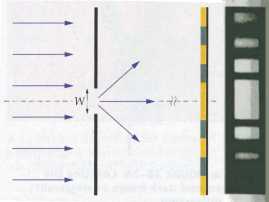
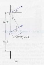
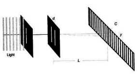
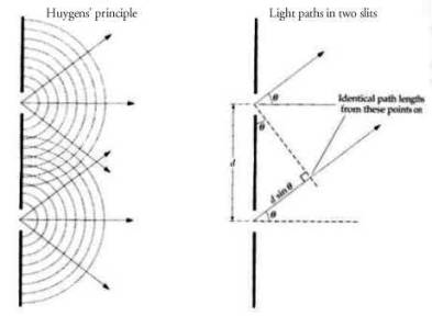
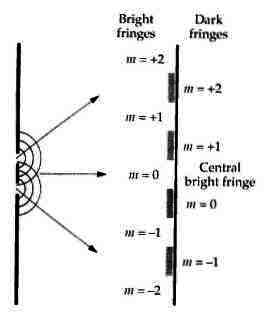

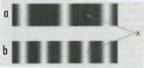
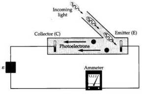
 g.
g.